Attitional Results
Menu
- Computational complexity
- Block size of GDM
- GDM
and filtered GDM
- VSM, LCM, and GDM Examples for NRID
- Normalization strategies
- Results for RetargetMe Dataset
- The proposed adaptive weighting function
- Limitation
Computational Complexity
Our method takes about 115 secs
for
assessing an image (retargeted from 768x512 to 576x512) on a quad-core
(Intel
i7) personal computer with 16GB Ram using Matlab without any code
optimization.
In our method, SIFT flow estimation, saliency map estimation, and the
rest
operations consumes about 85%, 12%, 3% of computation, respectively.
The
complexity of the most dominating operation SIFT flow estimation for an
NxN image for one iteration is
O(N2log2N) [20]. The other
operations are of O(N2) complexity.
Block size of GDM
The main reason is that the size of a geometric deformation region
(i.e., with relatively large local variance value of SIFT flow vectors)
is usually not small. Therefore patches with a reasonable range of size
can still capture the local variations of SIFT flow vectors. Besides,
the variance values of the patches in GDM are all normalized to [0,1],
which leads to a stable range of variance values regardless of the
patch size.
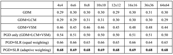
Although the rank correlation performance of the proposed
metric is not sensitive to the patch size, the patch size does affect
the computation and memory costs, and the granularity of perceptual
distortion visualization and localization
Table 1. Rank correlation of objective and subjective measures for the
second dataset dataset over various block sizes and different
combination of the proposed GDM, VSM, LCM, and SLR metrics.
GDM
& Filtered GDM
Similarly,
to make the SIFT flow map more reliable, small isolated noises (say,
less than 2x2) should be removed from the map, whereas larger defects
(i.e., those with significant local variance due to retargeting
distortion) should be enhanced. To this end, we perform anisotropic
diffusion filtering prior to the patch-based local variance analysis as
illustrated in Fig. 1 (we already put it in our project page but not in
the revised manuscript due to limited space).
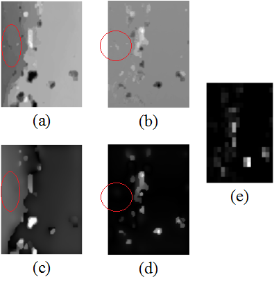
Fig. 1.Illustration
of the effect of the anisotropic diffusion filter. (a) and (b): The
horizontal and vertical components of SIFT flow map; (c) and (d): The
filtered versions of (a) and (b) using the anisotropic diffusion
filter; (e) the resulting GDM map after block-wise local variance
analysis.
VSM,
LCM, and GDM Examples (our dataset)
We
select two different images to show their VSM, GDM, and LCM of the
retargeted images. Note that the VSM are the same for five retargeted
images because the VSM is estimated from original image (the size of
the VSM, GDM, and LCM have to the same). The GDM captures the local
distortions for retargeted images. For example, the retargeted image
using shift-map have largest distortion (PGD) because the local
variation is relevantly large, compared to other retargeted images.
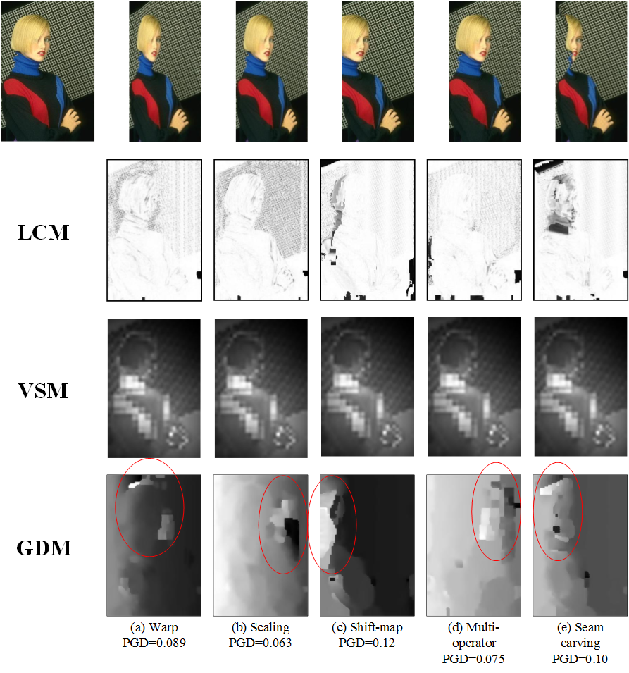
Fig.2. The proposed LCM, VSM, and GDM for test image 3 with its
retargeted images.
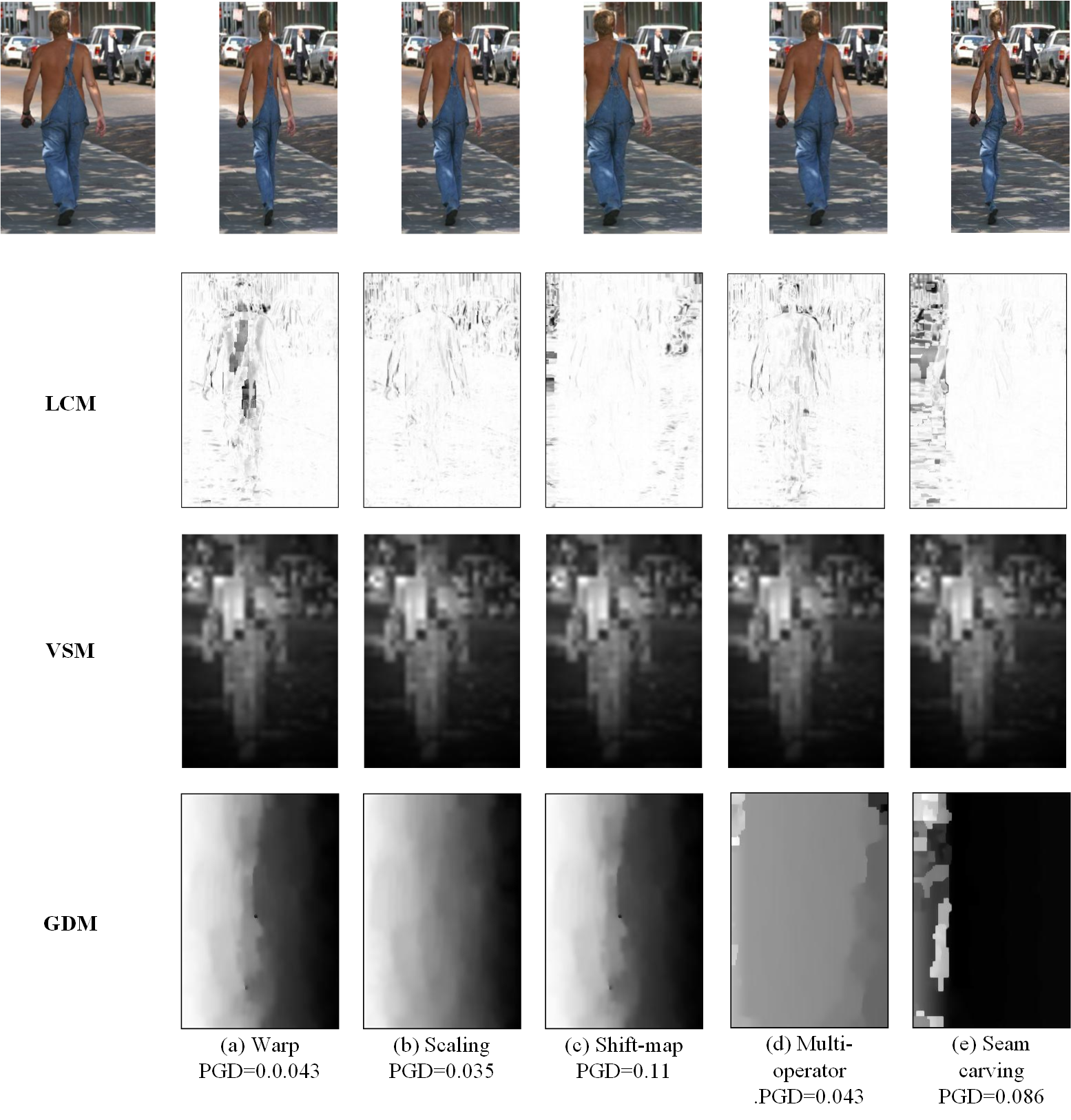
Fig.3. The proposed LCM, VSM, and GDM for test image 5 with its
retargeted images.
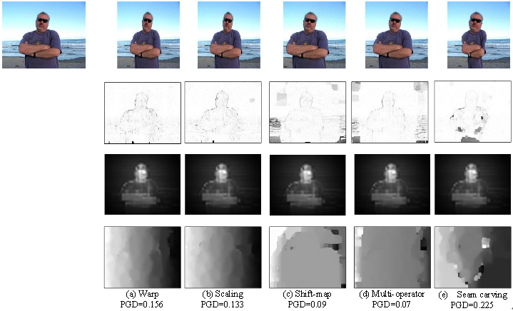
Fig.4. The proposed LCM, VSM, and GDM for test image 12 with its
retargeted images.
Normalization strategies
We have performed an experiment to compare two
normalization schemes for each test image. The first normalization
scheme (see Table 2:N1) is to normalize the metrics of a retargeted image based
on the minimal and maximal metric values among the patches “in
the image itself” (the one we are using). The second scheme (see
Table 2:N2) is to normalize the retargeted versions of a test image
based on the minimal and maximal metric values among the patches
“in the set of all retargeted versions” (8 versions for RetargetMe
and 5 versions for the second dataset) of the
image. Since we use the same VSM for all retargeted versions of a test
image, the second scheme is only applied to GDM and LCM. Our results
show that the performance difference between the two schemes are very
minor and negligible. Since the complexity of the first scheme is
lower, we keep the scheme unchanged.
Table 2. Rank
correlation of objective and subjective quality comparison over
different normalization strategies.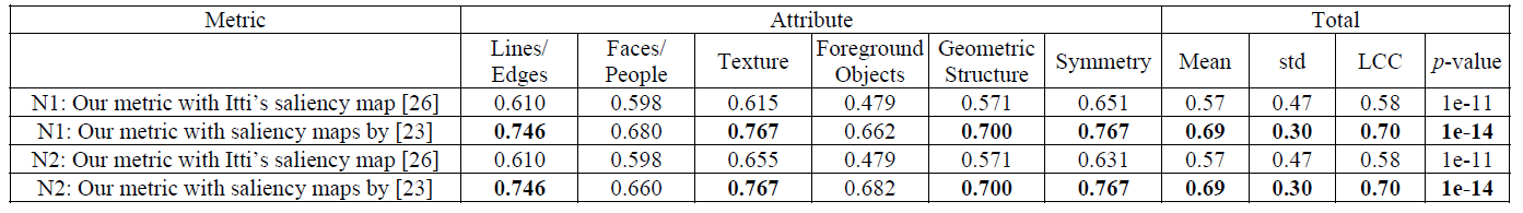
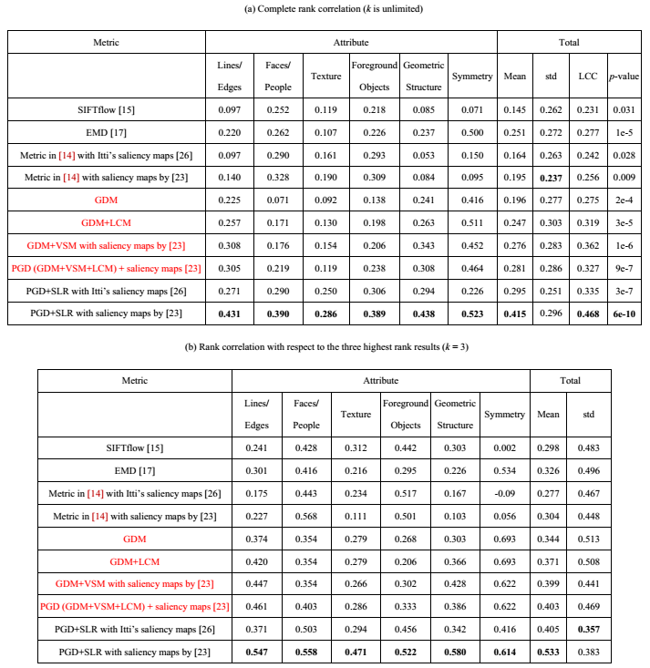
Results for RetargetMe
Dataset
Table 3. Rank correlation of objective and subjective
measures for the RetargetMe dataset [3].
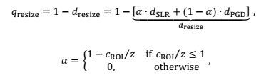
The proposed adaptive weighting function
Our adaptive fusion scheme
is based on the assumption that a saliency map containing too many
isolated
salient regions usually indicate the image has no dominating salient
objects/regions
or it is not reliable. In this case, the SLR metric will become less
important
and its weight should be discounted as in equations (9) and (10).
Otherwise,
the SLR metric takes a higher weight if there is dominating salient
regions.
Although the assumption may not apply to all kinds of
images perfectly, the
method works well for most of the images in the two datasets used using
the
saliency detection schemes in [1] and [2] as reflected in the
comparison of
adaptive weighting and fixed weighting shown below, where the blue
lines
indicate the rank correlation values with α varying from 0 to 1
with an
interval of 0.1.
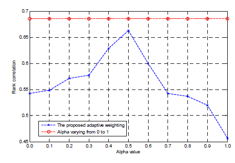
Fig. 5. Rank correlation value
versus the weight value between SLR and PGD.
Limitation
Our method also has its limitations. First, the accuracy
of the SIFT flow map has significant impact on the accuracies of the
PGD and SLR metrics. For some images with lots of repeated texture
patterns or very smooth areas, the SIFT flow estimation may not work
well for some parts of the images as it may find many incorrect
correspondences in these parts. Usually, the inaccuracy of SIFT flow in
the smooth area does not have much impact on the accuracy of the
proposed metric since the geometric distortion and information loss are
visually less significant in smooth areas. But for the texture regions,
the inaccuracy does matter. For the 10 highly textured images in the
two datasets including 72 test images, the rank correlation values are
all below the average. Besides, the proposed method may fail when the
saliency detection result is not reliable which usually happens if an
image does not contain significant salient objects/regions with an
enough large size or the scene is too complex (see Fig.6). Unreliable
saliency map will reduce the accuracies of PGD (due to unreliable
VSM) and SLR metrics.
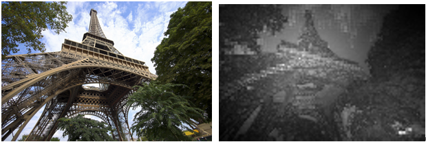
Fig. 6. An example of inaccurate saliency map.
Reference
[1] Y. Fang, W. Lin, Z. Chen, and C.-W.
Lin, “Saliency detection in the compressed domain
for adaptive image retargeting,” IEEE Trans. Image Process. vol. 21, no. 9, pp. 3888−3901, Sept. 2012.
[2] L. Itti, “Automatic foveation for video
compression using a neurobiological model of visual attention,” IEEE
Trans. Image Process., vol. 13, no. 10, pp. 1304-1318, Oct. 2004.
[3] RetargetMe
Benchmark [Online]. Available: http:// http://people.csail.mit.edu/mrub/retargetme/index.html